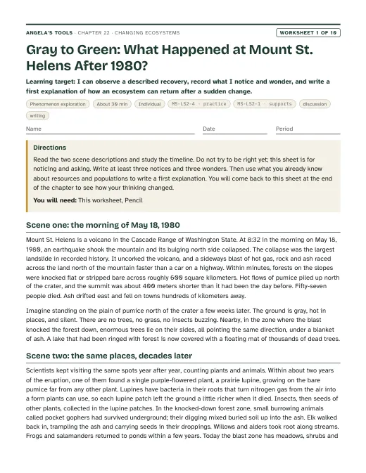
Gray to Green: What Happened at Mount St. Helens After 1980?
I can observe a described recovery, record what I notice and wonder, and write a first explanation of how an ecosystem can return after a sudden change.
Chapter 22 · Unit 7: Resources in Ecosystems · Segment 3
How do ecosystems change over time, and how can we use evidence to argue that a change to one part of an ecosystem affects the populations living there?
Students figure out that every ecosystem is a dynamic system that is always changing, sometimes over centuries as a pond fills in and sometimes in minutes when a volcano erupts, and that living things rebuild a damaged place through ecological succession. They use the 1980 eruption of Mount St. Helens and its decades of recovery as an anchor, then trace how changing one living part (a prairie dog town) or one nonliving part (a beaver dam, river sediment) shifts resources and sends ripples through many other populations. The core skill is argument from evidence: students learn to compare places with and without a change, read before-and-after data, and decide which claims the evidence actually supports. The chapter closes with the engineering strand, where criteria and constraints shape how engineers rebuild coastal wetlands.
Estimated class time: presentation about 140 minutes · worksheets about 425 minutes in total · labs 4 sessions. Eight 50-minute periods: one for the phenomenon and dynamic systems; one for succession and the Lab 1 mystery; one for the Lab 1 reveal, living-part changes and the reading; one for the Lab 2 string web; one for nonliving-part changes and the data worksheet; two for Lab 3 (field day and data day); and one for the argument checklist, the engineering strand and the closing slides. W2, W3, W6 and W7 work as homework; W8 and W9 can run as extension days or stations; W10 is the quiz.
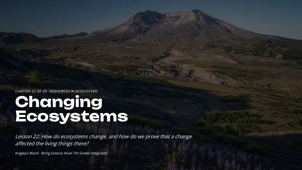
On the morning of May 18, 1980, the north side of Mount St. Helens in Washington State collapsed in the largest landslide ever recorded. A sideways blast of hot gas and rock flattened or scorched forests across roughly 600 square kilometers, and flows of hot pumice buried the valley north of the crater under a bare gray plain. Photographs from that summer show a landscape that looks like another planet: no trees, no grass, no visible animals. Photographs of the same valley forty years later show meadows of purple lupine, thickets of willow and alder, herds of elk, and ponds full of frogs. No one planted the plain; it was left to recover on its own. How did life come back, where did it come from, and why is the new ecosystem still not the old forest?
Notice and wonder prompts
California NGSS, Grade 7 Preferred Integrated Course Model. Each entry says whether this chapter's work assesses the performance expectation, gives practice toward it, or supports it as background; the resource lists below repeat this for every worksheet and lab.
Construct an argument supported by empirical evidence that changes to physical or biological components of an ecosystem affect populations.
This is the chapter's performance expectation. Students construct arguments supported by empirical evidence in Lab 3 (their own pooled disturbed-versus-undisturbed plot data), the Lab 2 closing argument (real survey counts of burrowing owls on active and inactive prairie dog colonies), W6 (a CER from with-and-without and before-and-after plot data), the W8 individual argument from published prairie dog findings, and W10 items 9 and 12. W5 and the slide 20 task practice reading the same kinds of data, and Lab 1 and the Lab 2 string-web trials practice the reasoning with observation cards and a model before students use measured data.
Define the criteria and constraints of a design problem with sufficient precision to ensure a successful solution, taking into account relevant scientific principles and potential impacts on people and the natural environment that may limit possible solutions.
The lesson's engineering spread shows how criteria and constraints shaped two different wetland-rebuilding designs in Louisiana. Students identify criteria and constraints in the W9 transfer task and the slide 25 discussion, but they do not define a full design problem with precision, so the role is practice rather than assesses.
Evaluate competing design solutions using a systematic process to determine how well they meet the criteria and constraints of the problem.
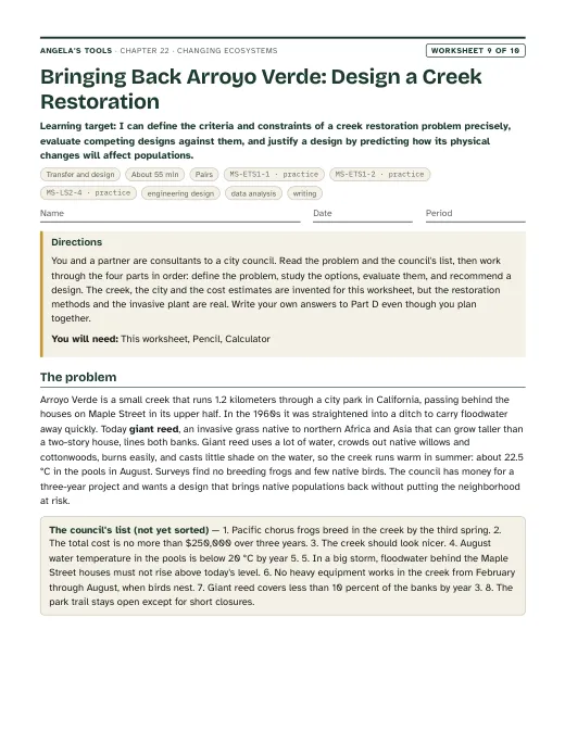
In W9 students evaluate five creek-restoration options and one combination systematically, eliminating any that break a constraint before scoring the rest against the criteria. The options and cost estimates are supplied rather than designed by students, so the role is practice. The slide 24 comparison of two Louisiana wetland designs previews the same reasoning.
Analyze and interpret data to provide evidence for the effects of resource availability on organisms and populations of organisms in an ecosystem.
Every cascading change in this chapter runs through resources: a beaver dam changes water depth and light, prairie dogs change shelter and soil, and succession changes soil and shade. Students use the resource-population relationship from Lesson 20 as background rather than producing new evidence for it.
Changing Ecosystems: how a damaged place stages its comeback. Original, editable slides with speaker notes: a phenomenon opener, learning targets, the chapter's concepts with diagrams, vocabulary in context, 3 checks for understanding, 2 discussion prompts, an application task, a misconception check, a synthesis and an exit ticket.

Ten different tasks, one per instructional blueprint. Each has a student PDF (low ink, US Letter), an editable DOCX, an HTML preview, and a separate teacher answer key with reasoning.
I can observe a described recovery, record what I notice and wonder, and write a first explanation of how an ecosystem can return after a sudden change.
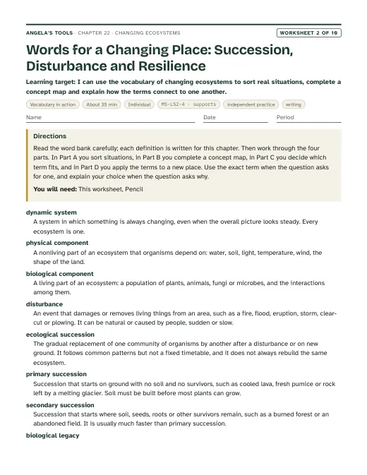
I can use the vocabulary of changing ecosystems to sort real situations, complete a concept map and explain how the terms connect to one another.
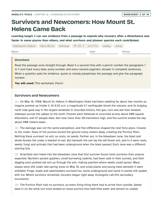
I can use evidence from a passage to explain why recovery after a disturbance was faster in some places than others, and what survivors and pioneer species each contributed.
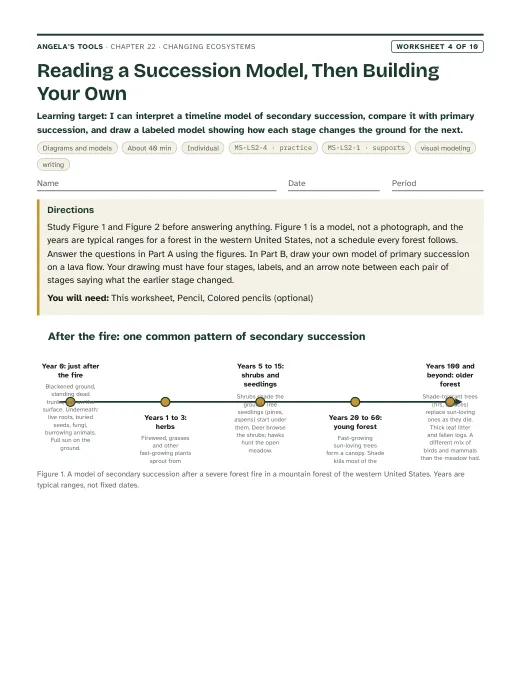
I can interpret a timeline model of secondary succession, compare it with primary succession, and draw a labeled model showing how each stage changes the ground for the next.
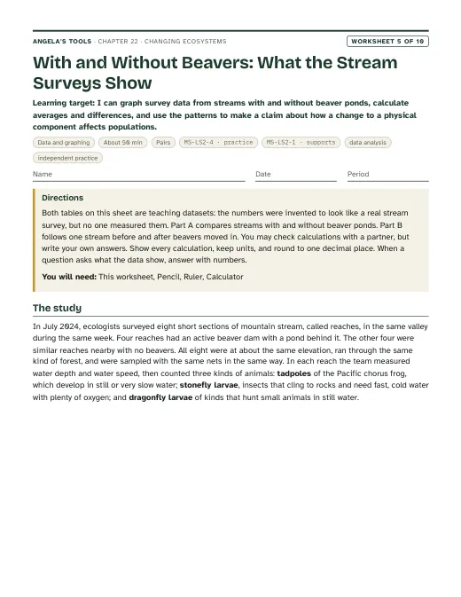
I can graph survey data from streams with and without beaver ponds, calculate averages and differences, and use the patterns to make a claim about how a change to a physical component affects populations.
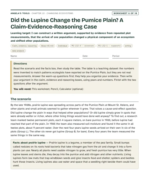
I can construct a written argument, supported by evidence from repeated plot measurements, that the arrival of one population changed a physical component of an ecosystem and shifted other populations.
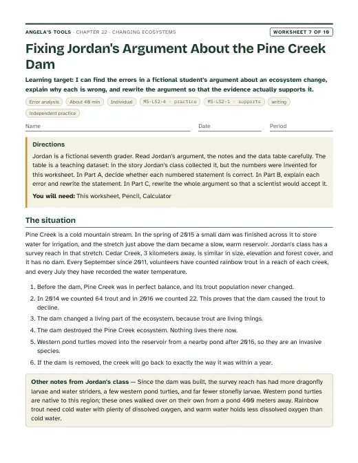
I can find the errors in a fictional student's argument about an ecosystem change, explain why each is wrong, and rewrite the argument so that the evidence actually supports it.
I can sort evidence about prairie dogs by the population it describes and by how strong it is, and use the strongest evidence to argue how losing a keystone species affects other populations.
I can define the criteria and constraints of a creek restoration problem precisely, evaluate competing designs against them, and justify a design by predicting how its physical changes will affect populations.
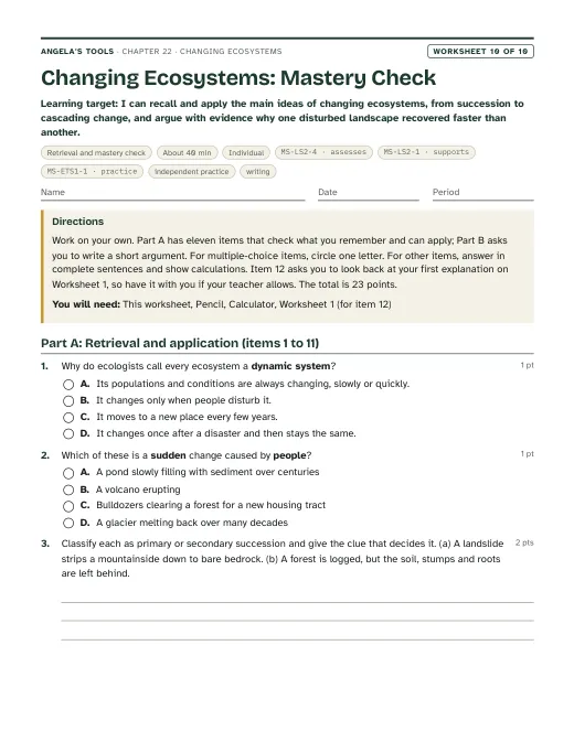
I can recall and apply the main ideas of changing ecosystems, from succession to cascading change, and argue with evidence why one disturbed landscape recovered faster than another.
Three different investigation approaches. Each has a teacher guide (purpose, materials with quantities, estimated cost, prep, safety, procedure, expected observations, debrief, answer key, assessment criteria, accessibility adaptations, low-cost alternative) and a student recording sheet.
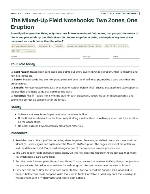
Using only the clues in twelve undated field notes, can you put the return of life in two places hit by the 1980 Mount St. Helens eruption in order, and explain why one place recovered so much faster than the other?
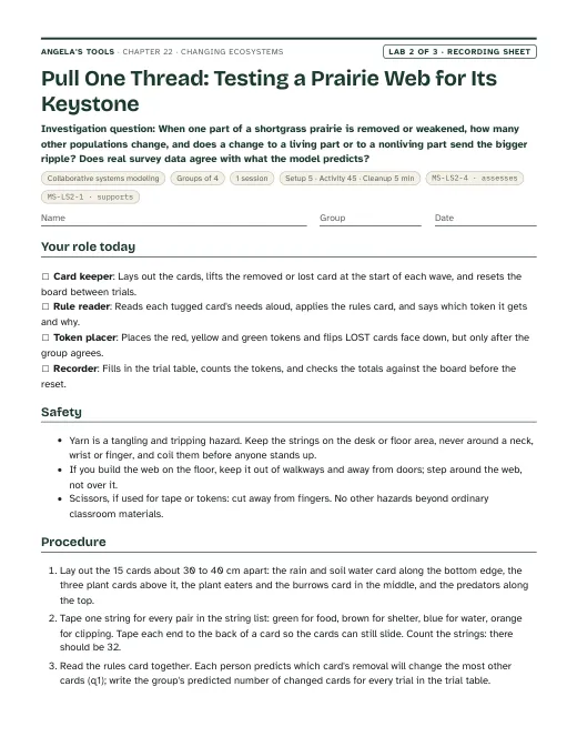
When one part of a shortgrass prairie is removed or weakened, how many other populations change, and does a change to a living part or to a nonliving part send the bigger ripple? Does real survey data agree with what the model predicts?
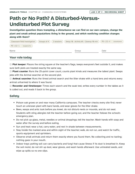
Does trampling, a disturbance we can find on our own campus, change the plant and small-animal populations living in the ground, and which nonliving condition changes along with them?
Materials overview: No chemicals and no heat. Lab 1 uses printed field-note cards, timeline strips and sticky notes. Lab 2 uses printed web cards, pre-cut yarn in four colors, masking tape and paper tokens. Lab 3 uses string squares, a meter stick, hand lenses, paper plates, bottomless plastic cups, water, a timer and gloves; the indoor alternative needs four shallow trays, potting soil and untreated fast-growing seeds started ten to fourteen days ahead. Printed before-and-after photographs of Mount St. Helens (public domain from the U.S. Geological Survey) make the phenomenon vivid.
Review status: reviewed · 2026-10-19 · Mount St. Helens facts checked against USGS: 8:32 a.m. magnitude 5.1 earthquake on May 18, 1980, largest debris avalanche in recorded history, about 600 square kilometers (230 square miles) devastated with damage reaching about 30 km (19 miles), 57 deaths, summit about 400 m lower, ash above 24 km, monument created 1982. The phenomenon, slide 2 and the W1 timeline now say forests were 'flattened or scorched/killed' (the 600 square kilometers include standing dead forest), and slide 2 notes, accuracy note 10 and the lateral-blast reference no longer say trees were flattened 30 km out. The dead USGS eruption URL was replaced. First lupine: a 2000 Washington State University report says 1981 and a magazine account of the ecologist credited with the find says June 1982, when the plant already had seedlings. W1 (scene, q1 key, notes) and W3 (paragraph 4, notes; passage now 690 words) say 'within about two years' instead of 'within two years'; slide 11 notes and accuracy note 10 no longer call the 1982 source 'the finder's own account'. Survivor and biological-legacy statements match the USGS monument ecology page. Re-solved every numeric, multiple-choice, true/false and table item in W1-W10 and Labs 1-3; W5 beaver means (115.0/30.0 cm, 5.5/46.0 cm/s, 60.0/5.0, 3.0/38.0, 17.5/2.5), ratios 12 and 7, 92.1 percent, reach J 4.75 to 57.0 and 40.0 to 4.3; W6, W7, W9 matrix (A 4, B2 3, D 2, A+B2 6, B1 and C eliminated), W10 total 23, Lab 1 rates and Lab 3 practice means (36.0/74.0 percent cover, 5 of 6 pairs; 215/60 s, about 3.6 times) are all correct. Fixed: W3 q7 key cited paragraph 7 as 'earlier' evidence (now paragraph 6); W7 q5 and q9 keys now treat 2015 (18 °C) as the transition year. Lab 2 string web re-simulated independently from the card needs, the 32-string list and the wave rules: prairie dogs 12 changed (8 in wave 1, then owls and cottontails, then grasshoppers and deer mice; burrows, ferrets and owls LOST), bison 1, grasshoppers 7, drought 14 over three waves with none lost, and every single-removal total in the teacher notes matches; no MIXED card arises. Sidle and others (2001) confirmed: 582 colonies surveyed in 1998, owls on 307 of 444 active (69 percent) and 15 of 138 inactive (11 percent). q8(b) now says the wildflower UP prediction is for removing prairie dogs. Standards: MS-ETS1-2 (practice, caGrade 6-8) added to chapter.json to match W9's decision-matrix evaluation of given options, with ETS1.B added to threeDimensions; the MS-LS2-4 note now names the tasks that actually carry 'assesses' (Lab 2 closing argument, Lab 3, W6, W8, W10) and lists W5 and the slide 20 task as practice. caGrade is present and matches standards.json on every entry. Vocabulary trimmed from 13 to 12 by removing 'criteria and constraints', which L21, L27, L29 and the earlier engineering chapters teach as vocabulary; the ideas stay on slide 24 and in W9 and W10, and the remaining twelve terms all appear in the W2 word bank. Consistency: the period 7 and 8 sequence now assigns W7 before the exit ticket and W6 after it, so the slide 28 advice (students who miss question 3 revisit W7 before writing W6) can be followed; W6 and W7 notes match. Slide 27 notes no longer imply lab evidence goes into W6. Lab 1 debrief corrected: the cover slopes are equal from 2000 to 2010 and the pumice line is steeper after 2010. Other checks: giant reed (native to northern Africa and western and central Asia; Cal-IPC High; heavy water use, poor stream shading and warmer water, fire fuel) with the W9 origin wording corrected; prairie dog range about 5 percent of original (slide 14 notes reworded, plague added); ferret captures by 1987 and releases since 1991; plague about 1900; northern California bull kelp loss over 90 percent and the 2018 abalone closure; Wax Lake 1941; Caernarvon 1988-1991. No six-word run is shared with the lesson text; two five-word echoes about 'squirrels that live in large' groups were reworded. Labs 1 and 2 now say they have not been physically tested, like Lab 3.
Verified against the student edition of Bring Science Alive! 7th Grade Integrated (Student Edition). Printed page numbers appear in the book; PDF pages are the physical pages of the 524-page scan (printed + 36). The textbook is not reproduced on this site.
| Section | Printed pages | PDF pages | Used for |
|---|---|---|---|
| Introduction: the melting glacier and the lesson question | 284, 285 | 320, 321 | Lesson question, dynamic system and succession vocabulary, the glacier-forefield example of primary succession, publisher standards (MS-LS2-4, MS-ETS1-1). |
| 1. Ecosystems Change Over Time: gradual change, sudden change, succession | 286, 287 | 322, 323 | Pond-to-forest sequence, eruption as sudden change, natural versus human-caused disturbances, Lab 1 two-zone sequencing mystery, slides 5-11. |
| 2. Changes to Living Parts of Ecosystems: prairie dogs | 288, 289 | 324, 325 | With-and-without comparison as evidence, species that gain and lose, keystone idea, Lab 2 string web, slides 13-16. |
| 3. Changes to Nonliving Parts of Ecosystems: beaver dams | 290 | 326 | Water depth, water speed and light as nonliving resources; downstream effects; slides 17-19 and W4. |
| Key Science Concept: Ecosystem Changes Shift Populations | 291 | 327 | Before-and-after population comparison as a form of evidence; the slide 20 task uses an original simulated dataset in the same spirit. |
| 4. Rebuilding Wetland Buffers: criteria, constraints, Wax Lake and Caernarvon | 292, 293 | 328, 329 | Engineering strand: criteria versus constraints, why two places needed two designs, slides 24-25 and W9. |
| Lesson Summary | 293 | 329 | Check that the four big ideas (change over time, living parts, nonliving parts, engineering) are all covered in the synthesis slide. |